Recall that given two points in the plane, an ellipse can be defined as the collection of points whose sum of distances to the given points is constant. But here in the Prisoner’s Dilemma, we know there are more operations than just addition. (Remember Dilemma 4?)
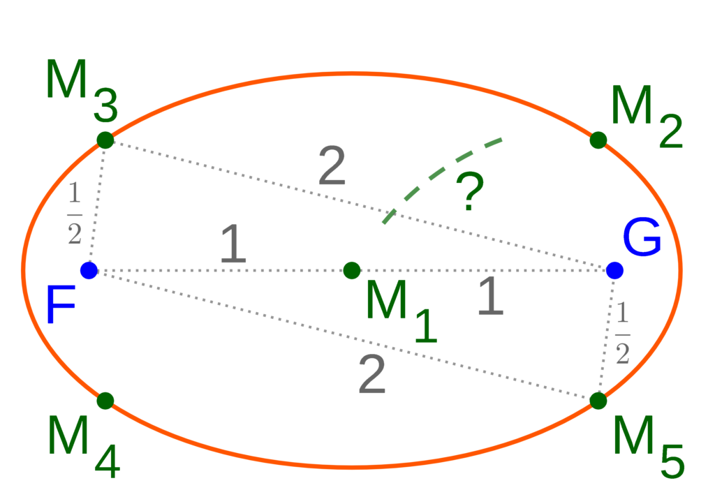
Figure 2: Five points (in green) on a curve of “constant distance product.” Where does the curve go between these points?
So suppose you are given points and a distance two units apart in the plane. We write just for the distance between points and in the plane (so for example, ). Describe the collection of all points in the plane such that As a start, figure 2 shows five of the points in this collection (four of which also happen to lie on the orange ellipse defined by ). You might also want to consider how the shape of this collection changes when you use a constant other than one; in other words, what does the collection of points such that look like for other values of ?
This problem originally appeared in the Prisoner’s Dilemma in the 2022 Fall issue of the PMP Newsletter. Solutions are no longer being accepted for this Dilemma.
Show solution?
Solution.
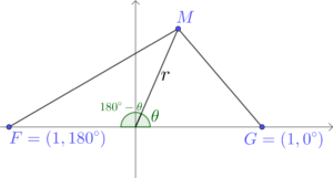
Figure 2: The point in polar coordinates.
PMP participants Chris Bistryski of Monroe, WA, William Jones of FCI Loretto, William Keehn, and Jesse Waite submitted solutions to this problem. As Mr. Keehn pointed out, it’s smoothest to work with polar coordinates; see Figure 2 for an illustration of the coordinates of a general point on the mullipse. We have by the Law of Cosines that Similarly, because ,
The definition of the curve we want is that , so we also have that Substituting and using the difference of squares, these observations mean that Finally, multiplying out, collecting terms, and using the cosine double-angle formula gives us:
Figure 3: Example Cassini ovals. Courtesy of desmos.com.
This last equation gives us a pleasantly simple (polar) equation for the mullipse. You can see it as the green curve in Figure 3. (An equation for it in Cartesian coordinates is which you can find by a similar process.)
As for what you get when the desired product 1 is replaced by some other constant , you can re-do the same derivation starting from to get the formula These curves for equal to 0.5, 0.75, 1, 1.25, and 1.5 are shown in Figure 3. In case you’d like to look up more information about them, the mullipse is more widely known as the “lemniscate of Bernoulli” and the whole family of curves created by varying the constant are called “Cassini ovals.”